3. Thermodynamics (ii) - Moist thermodynamics

3. Thermodynamics (ii) - Moist thermodynamics#

Our main conclusions from the last lecture were:

that hydrostatic force balance gives an excellent approximation to the observed global pressure dropoff with height
that dry adiabatic energy exchange as we lift a parcel from the surface temperature can only explain dropoff of temperature (with about 10 K/km) in the atmosphere’s lowest couple hundred metres.

We also argued that the premise that the vertical temperature distribution is set by the vertical mixing of air parcels is not the problem. Rather, we argued that we were missing some physics in our highly simplified, dry adiabatic situation. It turns out that to truly understand the vertical structure of temperature, we can’t assume the atmosphere is dry.

Note

Questions you should be able to answer at the end of this lecture:

What is energetically different about moist air than dry air?
Can I describe quantitatively when moist air saturates?
Where does a parcel’s lifting condensation level lie?
What is moist adiabatic ascent, and which variables are conserved in such a process?
Do I understand which principles set the moist adiabatic lapse rate?
Can I read a thermodynamic (skew T-log p) diagram, with moist processes?
Why is the globally averaged lapse rate so close to the moist adiabat?

Energy flows in moist air#

How is moisture an energy source for a parcel which is trying to rise? We said last lecture that for a parcel of mass $m$, the energy could be written as:

\[ E/m = gz + \frac{1}{2}u^2 + U/m \]

This is still true for moist air. But the internal energy $U/m$ of moist air is different than that of dry air. How? First, let’s recognise that because we are interested in the change of temperature (while an air parcel is moving), we are again interested in the flow of internal energy $dU/m$. So, let’s first revisit the conservation law we wrote down for $dU/m$,

\[ dU/m = Q_{a,E}/m dt + Q_r/m dt - pdV/m, \]

and express it in terms of enthalpy $H/m$ by using its definition $dH/m = dU/m + d(pV)/m$:

(28)#\[ dH/m = Q_{a,E}/m dt + Q_r/m dt + dp/\rho, \]

For dry air, $dH/m = c_{p_d} dT$, so we could directly relate $dT$ to $dp$, and (through hydrostatic balance), $dp$ to $dz$. But for moist air, we have to:

Partition $H/m$ across the dry air and water molecules, and
Account for the fact that heating the parcel does not always just increase its temperature. Specifcally, when the water in the parcel changes phase, applying a heating or a cooling to the parcel, will not go into increasing or decreasing the temperature. It will go into changing the phase of the water.

We can express this mathematically as follows. First, we split the composition of $m$ into contributions from dry air (subscript $d$), water vapour (subscript $v$), liquid water (subscript $l$) and solid water (ice, subscript $i$):

\[\begin{split} m & = m_d + m_v + m_l + m_s \\ 1 & = \frac{m_d}{m} + \frac{m_v}{m} + \frac{m_l}{m} + \frac{m_s}{m} \\ & = q_d + q_v + q_l + q_s \\ \end{split}\]

In the last line, we defined the “mass fractions” $q_x$[1] of dry air ($q_d$), water vapour ($q_v$), liquid water ($q_l$) and ice water ($q_i$)[2]. For this air mixture, changes in $H/m$ satisfy:

(29)#\[ dH/m = c_{p_m}dT + L_vdq_v - L_fdq_i, \]

where:

$c_{p_m}$ is the specific heat at constant pressure of moist air in J/kg/K (we will assume $c_{p_m} \approx c_{p_d}$, which is reasonable for what we’re trying to do here). $c_{p_m}dT$ expresses changes in heat through the moist air’s temperature. This is therefore called “sensible heat”.
$dq_v$ expresses a positive phase change into water vapour (and $d q_i$ into ice). The “latent heat of vaporisation” $L_v$ (in J/kg) tells us how much energy is expended to condensate 1 kg of water vapour into liquid water, or evaporate 1 kg of liquid into vapour (similarly, $dq_i$ scales the “latent heat of fusion” $L_f$). This heat is called “latent” (meaning “hidden”), because it’s hidden until the phase of water changes.

For this course, we take eq. (29) as given. However, it involves several non-trivial choices and approximations, which affect our further work (for example, why doesn’t $dq_l$ appear?). Ask me after the lecture if you are interested in knowing more about these fundamental thermodynamics.

Putting together eqs. (28) and (29), the new energy conservation equation for our moist air parcel states:

(30)#\[ c_{p_m}dT + L_vdq_v - L_fdq_i = Q_{a,E}/m dt + Q_r/m dt + dp/\rho. \]

If we raise the parcel adiabatically ($Q_{a,E} = Q_r = 0$) and assume it is in the same hydrostatic equilibrium as its environment ($dp/\rho=dp_e/\rho_e=-gdz$):

(31)#\[ -c_{p_m}dT - L_vdq_v + L_fdq_i = gdz. \]

So, to give the parcel potential energy $gdz$ in a situation without phase change, we have to expend $-c_{p_m}dT\approx-c_{p_d}dT$ of its sensible heat. This gives us the result from last time: $dT/dz = -c_{p_d}/g \approx 10$ K/km for such a parcel. But if $-dq_v$ of the parcel’s water vapour condenses over $dz$ ($-dq_v$ is a sink of water vapour, so it denotes condensation into liquid water), we can also invest the latent energy $-L_vdq_v$ into giving the parcel its potential energy (similarly, freezing $dq_i$ of the water gives another heat source). That is, for condensating parcels, the temperature drops off with height less rapidly. And that is exactly what we observe in the global troposphere: It is determined by rising motion in cloudy parcels.

To turn these observations into a quantitative estimate for the tropospheric lapse rate, we have to answer two questions:

When will water begin to condensate (or freeze)?
How much water will actually condensate and heat the parcel, when raising it a distance $dz$?

When will water begin to condensate?#

Saturation#

Let’s put a dry parcel directly on top of the ocean, close it off on all sides, and hold it at a pressure $p$ and temperature $T$. Water molecules will now evaporate into the parcel (e.g. through diffusion). In turn, some of the molecules will condensate back to the ocean. The parcel will get a vapour density $\rho_{v}$, exerting a partial “vapour pressure” $e=\rho_vR_vT$. If we wait long enough, the rates of condensation and evaporation from the surface will come in balance. The parcel is now “in equilibrium”, or “at saturation” with respect to the ocean surface: $\rho_v=\rho_{vs}$, and $e=e_s$: The relative humidty $e/e_s=\rho_v/\rho_{vs}\equiv{RH}=1$.

When we raise our parcel higher in the atmosphere, where we aren’t next to the ocean, it no longer has to be at saturation, i.e. $\text{RH}\leq 1$. But if it has $q_v$ kg water vapour per kg air, we can make it saturate, by lowering its temperature until $e=e_s$. We all know this intuitively, because cooling the near-surface air at night can condensate water vapour into dew on the grass. And going the other way, we’ve all seen how heating water in a pan makes it evaporate (at 100$^\circ$C at surface pressure, to be precise).

The Clausius-Clapeyron equation#

This relationship between the vapour pressure at which the air saturates $e_s$ (in Pa) and temperature (in K), is given by the “Clausius-Clapeyron” equation:

(32)#\[ \frac{1}{e_s}\frac{de_s}{dT} = \frac{L_v}{R_vT^2}. \]

This equation tells us something pretty fundamental about water in the atmosphere: At typical atmospheric temperatures ($T=288$ K), the fractional increase in water vapour the air can hold before it saturates $de_s/e_s$, increases with an increase in temperature $dT$ at a rate of $\frac{L_v}{R_vT^2}\approx\frac{2500\cdot 10^3}{461.5 \cdot 288^2}=0.0653$, or about 6.5 percent per K. This is called “Clausius-Claperyon scaling”. Put differently, the atmosphere’s capacity to hold water vapour before it condensates increases exponentially with temperature, and it does so pretty fast.

To solve eq. (32) for $e_s$, we have to integrate it, and to do that, we must make an assumption on $L_v$’s temperature dependence. If we just approximate it as a constant $L_v\approx 2500$ J/K at a reference temperature $T_0$, it can be solved by integrating away from that point:

(33)#\[\begin{split} \int_{e_{s0}}^{e_s} \frac{de_s'}{e_s} & = \frac{L_v}{R_v}\int_{T_0}^{T}\frac{dT'}{T^2} \\ \ln \frac{e_s}{e_{s0}} & = -\frac{L_v}{R_v}\left( \frac{1}{T} - \frac{1}{T_0} \right) \\ e_s(T) & = e_{s0}\exp\left({-\frac{L_v}{R_v}\left(\frac{1}{T} - \frac{1}{T_0} \right)}\right) \end{split}\]

Let’s plot this over the range of temperatures that occurs in the troposphere, around $T_0=273,15$ K, and $p=1000$ hPa. We also plot a slightly better approximation, called Tetens’ formula [3], which we will use in the course exercises and which appears in the reader:

\[ e_s(T) = 0.611 \times \exp\left(17.2694\times\frac{T - 273.16}{T - 35.86}\right) \]

Beware that this version takes as input the temperature in Kelvin and the pressure in kPa, but other versions exist which take the temperature in Celsius, or the pressure in Pa or hPa.

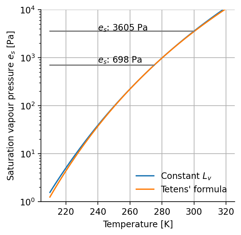
_images/12c10fe9609c589c1272b0ef874fbde810761d49a89791cfb3426e47a1ca385c.png

$e_s$ varies by almost four orders of magnitude over the troposphere! And the horizontal lines in the plot show that even for near-surface air, between the tropics ($T\sim 300$ K, $e_s \sim 3600$ Pa) and near the poles ($T\sim 275$ K, $e_s \sim 700$ Pa) there is a factor $3600/700\approx 5.1$ difference in how much water it can hold, before condensating it and raining it back down to the surface. This gives us intuition both for why near-surface air is moist and tropopause air is dry, and why the tropics are moist and the poles are dry. But it doesn’t tell us the balance of processes which achieve this yet.

The temperature and specific humidity of saturated air#

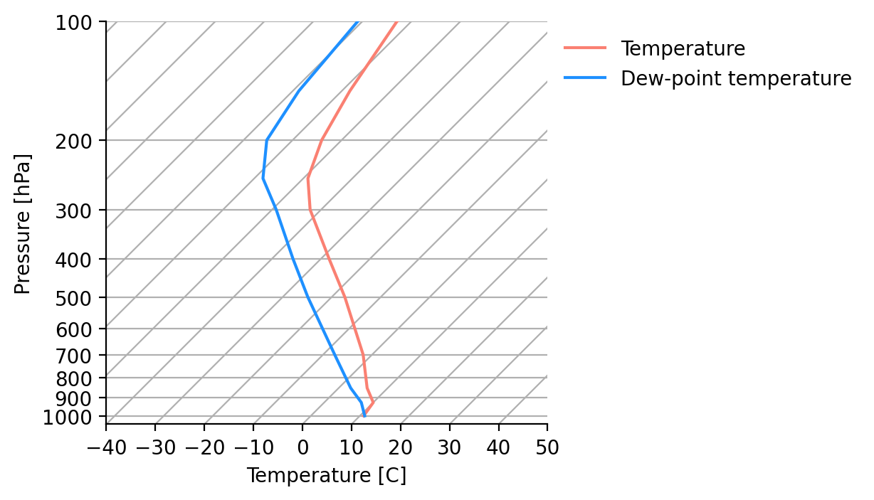
A different way to say all the above, is that for a parcel with vapour pressure $e$, we can define a temperature $T_d$ at which $e=e_s(T_d)$ ($RH=1$). $T_d$ is called the dew-point temperature. That is, if we know how much water there is in the parcel ($e$), we can solve eq. (33) to tell us at which temperature that water vapour will condensate. This is another way to express “how far we are from saturation”. We have plotted it for the average $e$ measured over the IGRA archive below, to confirm that on average, the global atmosphere is unsaturated: $T > T_d$.

_images/8cedc08b36743826e8591023900f663f92edce89c1982ce479aa0995d57a7a10.png

Often, the water vapour content is expressed not in vapour pressure $e$, but in fractions of the total mass ($q_v=m_v/m$). For those situations, we have to relate $e$ to $q_v$. We can do this using i) the gas law of the dry and moist phases ($p_d = \rho_d R_d T$, $e = \rho_v R_v T$) and ii) $p = p_d + e$ (Dalton’s law of partial pressures):

(34)#\[\begin{split} q_v & = \frac{\rho_v}{\rho_d + \rho_v} = \frac{\frac{e}{R_vT}}{\frac{p-e}{R_dT} + \frac{e}{R_vT}} = \frac{e}{\frac{R_v}{R_d}(p-e) + e} = \frac{R_d}{R_v}\frac{e}{p + e(R_d/R_v - 1)} \\ \end{split}\]

At saturation, $q_v \equiv q_s$, so:

(35)#\[ q_s(p, T) = \frac{R_d}{R_v}\frac{e_s(T)}{p + e_s(T)(R_d/R_v - 1)} \]

We can see from this relation that to determine $q_s$, we need to know both $e_s(T)$ and $p$. Still, the key point is that this relationship defines the dew-point temperature, so that $q_v = q_s(p, e_s(T_d))$: At a given pressure, if we know a parcel’s $q_v$, we can figure out at which temperature it saturates.

Because $p$ is usually 1-2 orders of magnitude greater than $e_s$ at the same $T$, we can to great approximation write[4]:

(36)#\[ q_s \approx \frac{R_d}{R_v}\frac{e_s}{p} \]

The lifting condensation level#

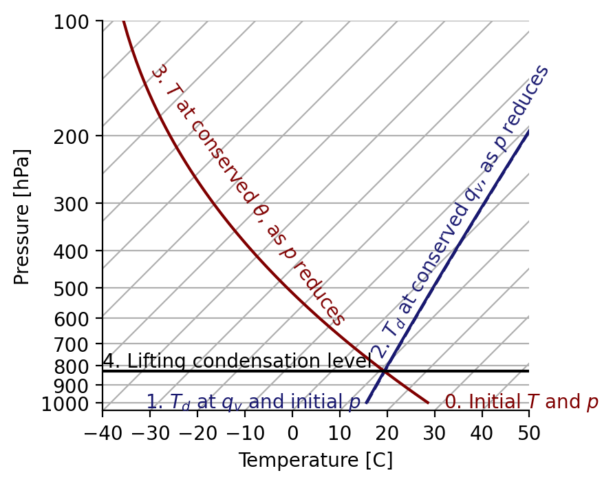
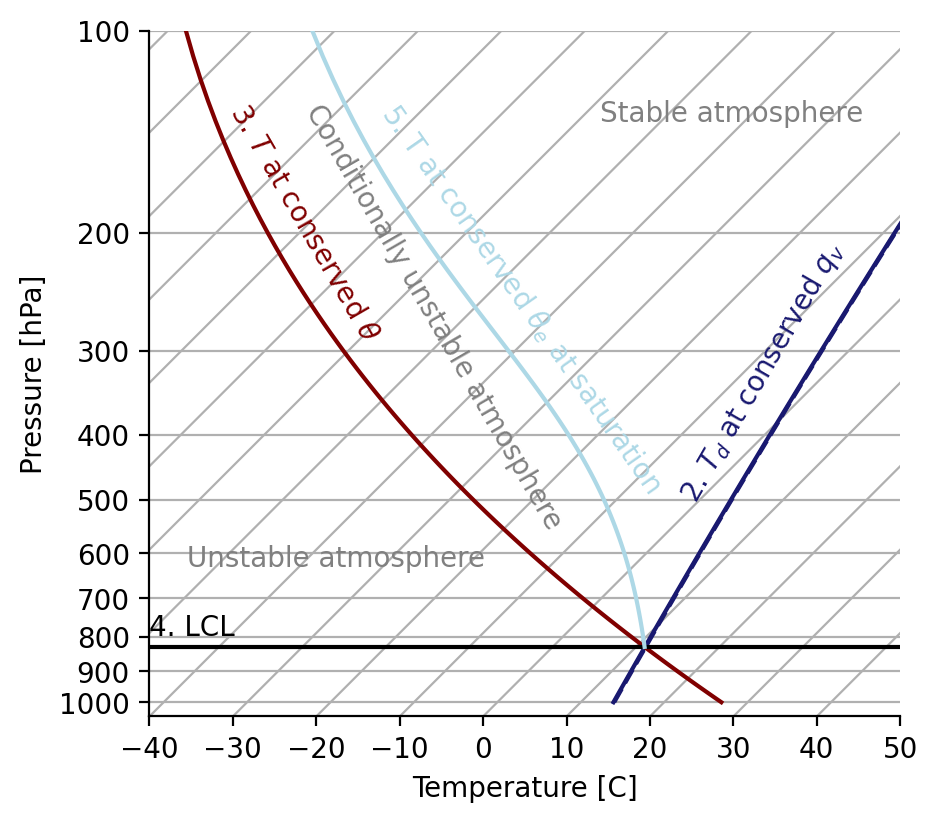
So, if we start to lift our parcel with $p$, $T$ and $q_v$ along a dry adiabat from a height $z_0$ while keeping $q_v$ constant, at what height will we reach $q_v=q_s$? This height is called the “lifting condensation level”, $z_{lcl}$. Although possible, writing an exact expression for $z_{lcl}$ is a bit beyond our course. But we can do it graphically in a skew $T$ - ln $p$ chart, using the following steps (see also the code and plot below):

Determine $T_d(q_v,p)$, by solving eq. (35) for $e_s(q_v, p)$, and then solving eq. (33) for $T_d$.
Repeat this calculation for $T_d$ for each $p$ we plan to lift the parcel to. If our parcel hits this line, we know that $q_v=q_s$, and we have saturation.
Actually move the parcel along a line of constant potential temperature $\theta$ (i.e. lift it dry adiabatically), until we hit the $q_s$ line.
That intersection is the pressure of the lifting condensation level. And in an atmosphere in hydrostatic balance, we can relate it to $z$ with the hydrostatic equation.

We have calculated these lines for a theoretical parcel below:

Show code cell source

Hide code cell source

# Parcel properties at its outset
p0 = 1e5 # Pa
T0 = 300 # K
qv = 0.01 # kg/kg

# Pressures we will lift the parcel to
p = np.linspace(1e5, 1e4, 100)

Rd = 287.05 # Dry air gas constant, J / kg / K
cpd = 1004 # Dry air heat capacity at constant pressure, J / kg / K

# Plot
fig = plt.figure()
skew = SkewT(fig, rotation=45)

# 0. Initial parcel T and p
skew.ax.text(0.8, 0.05, r'0. Initial $T$ and $p$', transform=skew.ax.transAxes, verticalalignment='top',
            c='maroon')

# 1. Initial dew-point temperature

# With full definition for qs
def e_sq(qs, p):
    return qs * p / (qs * (1-Rd/Rv) + Rd/Rv)

# With approximate definition for qs
def e_sq_approx(qs, p):
    return qs * p / (Rd/Rv)

Tdew0 = Tdew(e_sq(qv, p0))
skew.ax.text(0.1, 0.05, r'1. $T_d$ at $q_v$ and initial $p$', transform=skew.ax.transAxes, verticalalignment='top',
            c='midnightblue')

# 2. Tdew, as the parcel is lifted to lower p at constant qv
Tdew_qscst = Tdew(e_sq(qv, p))
Tdew_qscst_approx = Tdew(e_sq_approx(qv, p))
skew.plot(p/100, Tdew_qscst-T_trip, c='midnightblue')
skew.plot(p/100, Tdew_qscst_approx-T_trip, c='midnightblue', linestyle='--')
skew.ax.text(0.62, 0.9, r'2. $T_d$ at conserved $q_v$, as $p$ reduces', 
             transform=skew.ax.transAxes, rotation=60, verticalalignment='top', c='midnightblue')

# 3. Line of constant potential temperature
def Tpot(T, p):
    return T*(1e5/p)**(Rd/cpd)
Tpot0 = Tpot(T0, p0)
T_tpotcst = Tpot0 * (p/1e5)**(Rd/cpd)
skew.plot(p/100, T_tpotcst-T_trip, c='maroon')
skew.ax.text(0.1, 0.9, r'3. $T$ at conserved $\theta$, as $p$ reduces', 
             transform=skew.ax.transAxes, rotation=-54, verticalalignment='top', c='maroon')

# 4. Lifting condensation level, at the p where T_tpotcst and Tdew_qscst intersect
p_lcl = p[np.argmin(np.abs(T_tpotcst - Tdew_qscst))]
skew.ax.axhline(p_lcl/100, label='Lifting condensation level', c='black')
skew.ax.text(0.0, 0.15, r'4. Lifting condensation level', 
             transform=skew.ax.transAxes, verticalalignment='top', c='black')
skew.ax.set_xlabel('Temperature [C]')
_ = skew.ax.set_ylabel('Pressure [hPa]')
# plt.savefig('Figures/lcl-4.pdf',bbox_inches='tight')

_images/909a971b7fb210d3eb9b564f84db81fa1f4010fb084a1633973aca298464f47a.png

Moist adiabatic lapse rate#

Beyond the LCL, the parcel will condensate water vapour if we raise it further. So, if there are no external heat sources ($Q_{a,E}/m dt + Q_r/m dt=0$), the parcel is in perfect hydrostatic equilibrium with its environment ($dp/\rho=gdz$), and we ignore ice ($L_fdq_i=0$), we will have to spend some combination of $c_{p_m}dT$ and $L_vdq_v$ to raise the parcel:

(37)#\[\begin{split} c_{p_m}dT + L_vdq_v - L_fdq_i & = Q_{a,E}/m dt + Q_r/m dt + dp/\rho \\ c_{p_m}dT + L_vdq_v & = dp/\rho, \\ -c_{p_m}dT - L_vdq_v = gdz. \end{split}\]

In this situation, we can define an energy, called the moist-static energy (MSE), which remains conserved:

(38)#\[\begin{split} d\left(c_{p_m}T + L_vq_v + gz\right) = 0, \\ d \text{MSE} = 0. \end{split}\]

It is the moist analog of the dry-static energy $c_{p_d} + gz$, which we defined last time to be conserved over dry-adiabatic ascent at zero buoyancy. Our goal all along has been to find $dT/dz$ in the global atmosphere. Can we get it from this moist-adiabatically lifted parcel? Looking at eq. (38), it seems like we could, if we could relate the amount of water vapour condesated ($-dq_v$) in eq. (37) to the reduction in temperature ($-dT$) when we raise the parcel, and to $dz$. And since we are keeping the parcel in hydrostatic balance, we really want to relate it to $dT$ and $dz=-g/\rho dp$.

We know this is possible, because we just spent a lot of effort to convince ourselves that if the parcel is kept at saturation, i.e. $q_v = q_s$, then eq. (36) tells us that $q_s(T,p)$ only. So, as long as we are rising through a cloud, where $q_v=q_s$, $dq_v = dq_s$, which we can relate to $dp$ and $dT$ with the chain rule:

\[ dq_s = \frac{\partial q_s}{\partial p}dp + \frac{\partial q_s}{\partial T}dT \]

We next need to work out these two derivatives:

For $\partial q_s/\partial p$ at constant $T$, we can just use the definition $q_s \approx \frac{R_de_s}{R_vp}$ (notice we use it twice!): $$ \frac{\partial q_s}{\partial p} = -\frac{R_v}{R_d}\frac{e_s}{p^2} = -\frac{q_s}{p} $$
For $\partial q_s/\partial T$ at constant $p$, we have to take another step, because we know that it’s actually $e_s$ that depends on $T$ through the Clausius-Clapeyron equation (eq. (32)). We insert this, and get:

\[\begin{split} \frac{\partial q_s}{\partial T} & = \frac{R_d}{R_vp}\frac{d e_s}{dT} \\ & = \frac{R_d}{R_vp}\frac{L_ve_s}{R_vT^2} \\ & = \frac{R_de_s}{R_vp}\frac{L_v}{R_vT^2} \\ & = \frac{q_sL_v}{R_vT^2} \\ \end{split}\]

So:

\[ dq_s = -\frac{q_s}{p}dp + \frac{q_sL_v}{R_vT^2}dT \]

We can plug this into our energy conservation statement $c_{p_m}dT + L_vdq_v = dp/\rho$, gather terms, use hydrostatic equilibrium to relate $dp$ to $dz$, and solve for $dT/dz$:

(39)#\[\begin{split} c_{p_m}dT - dp/\rho + L_v\left(-\frac{q_s}{p}dp + \frac{q_sL_v}{R_vT^2}dT\right) & = 0 \\ \left(c_{p_m} + \frac{q_sL_v^2}{R_vT^2}\right)dT & = \frac{dp}{\rho}\left(1 + \frac{q_sL_v\rho}{p}\right) \\ \left(c_{p_m} + \frac{q_sL_v^2}{R_vT^2}\right)dT & = -gdz\left(1 + \frac{q_sL_v}{R_dT_v}\right) \\ \frac{dT}{dz} & = -\frac{g\left(1 + \frac{q_sL_v}{R_dT_v}\right)}{c_{p_m} + \frac{q_sL_v^2}{R_vT^2}} \\ \end{split}\]

And this has given us a new lapse rate, the moist adiabatic lapse rate.

Let us evaluate this lapse rate and compare it to our global radiosonde archive, and the dry adiabatic lapse rate we derived last lecture.

Mean dT/dz for moist adiabatic ascent: -0.007089509492679575

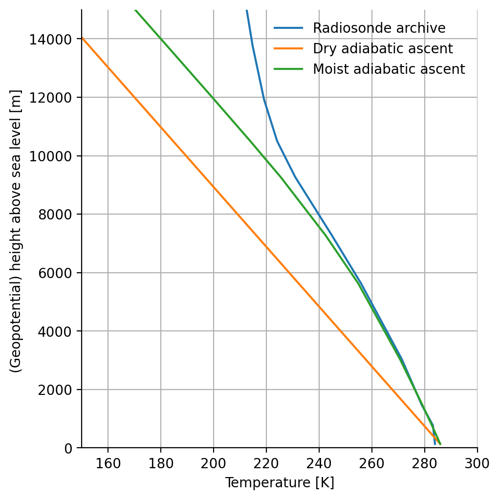
_images/523f5a095fb3b49db9b3ed949844b7d83e0dc9112d80e08168ec97edf022b1ce.png

This is not bad! The tropospheric temperature structure looks very much like that of a parcel lifted adiabatically from the surface at saturation with respect to liquid water.

Static stability of condensating parcels#

The argument for why it looks like this relies on buoyancy and mixing. To see it, we return to the vertical momentum equation we derived last time for a dry parcel. We say that a moist parcel (underscore $p$) ascending through a moist atmosphere (underscore $e$), using $p=\rho R_dT_v$ under the assumption that $p=p_e$, but $\rho\neq\rho_e$ satisfies:

\[\begin{split} \frac{dw}{dt} & = - \frac{\rho_p - \rho_e}{\rho_p}g = \frac{T_{v_p} - T_{v_e}}{T_{v_e}}g \\ & \approx \frac{T_{p} - T_{e}}{T_{e}}g. \end{split}\]

That is, we ignore the lightness of the water vapour in this approximation of the buoyancy[5].

Suppose we had a troposphere where the temperature reduced more quickly than a dry adiabat. Then parcels moving along a dry adiabat would be warmer than the atmosphere ($T_p > T_e$) at any height above the surface. We say that the atmosphere is statically unstable: The parcel would accelerate upwards until the tropopause, where it would quickly become negatively buoyant. We call the ascent of such parcels “dry convection”.

In a real atmosphere, the air parcels don’t ascend adiabatically, but actually mix some of their warm air into the environment. So, dry convection would warm the atmosphere, until it looks exactly like a dry adiabat ($dT/dz\approx-10$ K/km). Now, the atmosphere is neutrally stable to dry adiabatic ascent - if you warm a parcel by 1K at the surface and move it along a dry adiabat, it will always be 1K warmer. This is often the situation in the atmospheric boundary layer, as we discussed last lecture.

However, when temperature drops off less quickly than a dry adiabat ($dT/dz>-10$), we can still make parcels positively buoyant, if we warm them just enough to take them to the LCL: From there on, they saturate and lose temperature moist adiabatically ($dT/dz_m$). What is $dT/dz_m$? Eq. (39) shows that it actually depends on $T$, so it’s not constant with height. In fact, because $q_s$ becomes very small at the low temperatures high in the troposphere, $dT/dz_m\approx -g/c_p \equiv -dT/dz_d$ at high altitudes (you can see the lines orange and green lines become parallel in the plot above). However, a good average over the troposphere is $\Gamma_m\approx-7$ K/km. So an atmosphere where temperature drops off more quickly than $\sim$7 K/km is statically unstable to moist adiabatic, cloudy updrafts, called “moist convection”. These moist convective storms have $T_p>T_e$ over a large range of the troposphere. The temperature drops of at a rate between $dT/dz_d$ and $dT/dz_m$ (roughly 10 and 7 K/km), we say that the atmosphere is conditionally unstable, i.e. it is unstable, if the parcels are condensating.

As we will see in later lectures, radiation tends to cool the atmosphere, and pulls its temperature profile towards a dry adiabat. So, we often observe a conditionally unstable atmosphere, with lots of deep convection (especially in the tropics). By raining their condensed water vapour back to the surface, these storms heat the atmosphere, bringing the troposphere’s temperature profile towards that of the moist adiabat we observe in the global mean. There is no big energy source left in our atmosphere’s updrafts that could make the parcels much warmer than a moist adiabatic troposphere. Therefore, that is the temperature profile we observe.

If temperatures begin to drop off at an even slower rate than 7 K/km (and all the processes we have ignored could make that happen locally), parcels will always have $T_p<T_e$, and never rise on their own. We say that the atmosphere is statically stable in such a situation: There will be no convection, until other processes cool the atmosphere, or we put a giant heat source at the surface.

To illustrate all this, we have drawn a parcel ascent in the plot below. If we imagine atmospheric temperature profiles varying away from the same surface temperature, we can identify which of these atmospheres would be unstable, conditionally stable and stable to our parcel’s adiabatic ascent.

Show code cell source

Hide code cell source

# Parcel properties at its outset
p0 = 1e5 # Pa
T0 = 300 # K
qv = 0.01 # kg/kg

# Pressures we will lift the parcel to
p = np.linspace(1e5, 1e4, 100)

Rd = 287.05 # Dry air gas constant, J / kg / K
cpd = 1004 # Dry air heat capacity at constant pressure, J / kg / K

# Plot
fig = plt.figure()
skew = SkewT(fig, rotation=45)

# 2. Tdew, as the parcel is lifted to lower p at constant qv
Tdew_qscst = Tdew(e_sq(qv, p))
Tdew_qscst_approx = Tdew(e_sq_approx(qv, p))
skew.plot(p/100, Tdew_qscst-T_trip, c='midnightblue')
skew.plot(p/100, Tdew_qscst_approx-T_trip, c='midnightblue', linestyle='--')
skew.ax.text(0.7, 0.7, r'2. $T_d$ at conserved $q_v$', 
             transform=skew.ax.transAxes, rotation=60, verticalalignment='top', c='midnightblue')

# 3. Line of constant potential temperature
def Tpot(T, p):
    return T*(1e5/p)**(Rd/cpd)
Tpot0 = Tpot(T0, p0)
T_tpotcst = Tpot0 * (p/1e5)**(Rd/cpd)
skew.plot(p/100, T_tpotcst-T_trip, c='maroon')
skew.ax.text(0.1, 0.9, r'3. $T$ at conserved $\theta$', 
             transform=skew.ax.transAxes, rotation=-60, verticalalignment='top', c='maroon')

# 4. Lifting condensation level, at the p where T_tpotcst and Tdew_qscst intersect
index_lcl = np.argmin(np.abs(T_tpotcst - Tdew_qscst))
p_lcl = p[index_lcl]
T_lcl = T_tpotcst[index_lcl]
skew.ax.axhline(p_lcl/100, label='Lifting condensation level', c='black')
skew.ax.text(0.0, 0.15, r'4. LCL', 
             transform=skew.ax.transAxes, verticalalignment='top', c='black')

# 5. Line of constant equivalent potential temperature, at saturation, from the LCL
# Let metpy figure this out, because inverting equivalent potential temperature so it 
# expresses temperature in terms of pressure requires a root solver
from metpy.calc import moist_lapse
from metpy.units import units
T_ma = moist_lapse(p[index_lcl:] * units.Pa , T_lcl * units.K)
skew.plot(p[index_lcl:]/100, T_ma, c='lightblue')
skew.ax.text(0.3, 0.9, r'5. T at conserved $\theta_e$ at saturation', 
             transform=skew.ax.transAxes, rotation=-55, verticalalignment='top', c='lightblue')

# Where is the atmosphere stable, conditionally stable, or unstable?
skew.ax.text(0.05, 0.25, r'Unstable atmosphere', transform=skew.ax.transAxes, verticalalignment='top', c='grey')
skew.ax.text(0.2, 0.9, r'Conditionally unstable atmosphere', transform=skew.ax.transAxes,rotation=-60, verticalalignment='top', c='grey')
skew.ax.text(0.6, 0.9, r'Stable atmosphere', transform=skew.ax.transAxes, verticalalignment='top', c='grey')

skew.ax.set_xlabel('Temperature [C]')
_ = skew.ax.set_ylabel('Pressure [hPa]')
plt.savefig('Figures/lcl-final.pdf', bbox_inches='tight')

_images/a3064ed2c0813a308ec39bba1dce8e93399383ad7a9d3d40363f014ee500ef7a.png

Moist adiabatic motion in pressure coordinates - equivalent potential temperature#

When we drew the line of moist adiabatic ascent in pressure coordinates in the skew T - log p diagram above, we have actually not needed to assume the parcel is in hydrostatic equilibrium with the atmosphere, because we don’t have to invoke $dp=-\rho gdz$. This assumption was necessary to conserve MSE over the ascent. If we instead just integrate our energy equation (second line of eq. (37)) directly, from a reference temperature $\theta_e$ (called the equivalent potential temperature), a reference pressure $p_0$ and a reference $q_v=0$, the we get:

\[\begin{split} c_{p_m}dT + L_vdq_v & = dp/\rho, \\ \frac{dT}{T} & = \frac{R_d}{c_{p_m}}\frac{dp}{p} - \frac{L_vdq_v}{c_{p_m}T} \\ \int_{\theta_e}^{T}\frac{dT}{T} & \approx \frac{R_d}{c_{p_m}}\int_{p_0}^{p}\frac{dp}{p} - \frac{L_v}{c_{p_m}T}\int_{0}^{q_v}dq_v \\ \ln \left(\frac{T}{\theta_e}\right) & = \frac{R_d}{c_{p_m}}\ln\left(\frac{p}{p_0}\right) - \frac{L_vq_v}{c_{p_m}T} \\ \frac{T}{\theta_e} & = \left(\frac{p}{p_0}\right)^{\frac{R_d}{c_{p_m}}}\exp\left(-\frac{L_vq_v}{c_{p_m}T}\right) \\ \theta_e & = T\left(\frac{p_0}{p}\right)^{\frac{R_d}{c_{p_m}}}\exp\left(\frac{L_vq_v}{c_{p_m}T}\right) \\ & = \theta\exp\left(\frac{L_vq_v}{c_{p_m}T}\right) \end{split}\]

Here, in the second line we assume that $L_v$ and $T$ are constant when $dq_v$ changes, and we have used logarithm rules. We have also again neglected the virtual effect of water vapour. Also, $\theta_e$ has an analogous meaning for moist air as $\theta$ did for dry air in the previous lecture: It is the temperature you’d get if you brought an air parcel adiabatically from pressure $p$ to $p_0$, and brought its water vapour from $q_v$ to zero (e.g. by condensating all of it).

If we keep our air parcel at saturation when raising it adiabatically (i.e. with $-dp$), then $\theta_e$ remains conserved, for the same reason that MSE (kept at saturation) remained conserved with $dz$ when it is in hydrostatic equilibrium: We are simply converting latent energy into potential energy. So long as you keep the assumptions under this hydrostatic conversion in mind (see the next section if you’re interested), you can actually just think of $\theta_e$ as measuring the same as MSE$/c_{p_m}$.

Bonus (not part of the course)#

What we have ignored, and the extent to which it matters#

In the above, we made the following simplification of our general statement of an atmospheric energy flow:

\[\begin{split} c_{p_m}dT + L_vdq_v - L_fdq_i & = Q_{a,E}/m dt + Q_r/m dt + dp/\rho \\ c_{p_m}dT + L_vdq_v & = dp/\rho. \end{split}\]

What about the terms we ignored? Do they matter? For actual ascending parcels in the atmosphere:

It remains reasonable to assume radiation doesn’t heat or cool the parcel. The globally avereaged atmosphere cools radiatively at a pretty constant rate of around 2.5 K/day, which in energetic terms is $2.5\cdot c_{p_m}/(24\cdot 3600)=0.02$ W/kg. Air ascending through the atmosophere, even at 1 m/s (which is typical for turbulent overturning in the boundary layer), gains potential energy at $gdz/dt=10$ W/kg, so on the order of 100 times faster. Radiation does matter in clear skies, where the air descends at speeds which match the energy from this radiative cooling, while conserving dry-static energy.
We can often not ignore sinks of $H/m$ from mixing the parcel with the environment. Real parcels entrain air from their environment as they ascend, through turbulent mixing. The $q_v$ of this environmental air $q_{v_e}$ is usually lower than the $q_{v}$ of the parcel, $q_{v_p}$ (this is true by definition if the parcel is saturated and the environment isn’t, at the same $p$ and $T$). Therefore, over a distance $dz$, entrainment with a rate $\epsilon$ (in 1/m) reduces the parcel’s $q_v$ by $dq_{v_e} = (q_{v_e} - q_{v_p})\epsilon dz$. This reduction in $q_v$ can now not be spent on releasing heat through condensation, i.e. it reduces $L_v dq_v$ to $L_v(d q_v - dq_{v_e})$, and there is less energy available to lift the parcel. This matters when trying to predict e.g. how vigorous a thunderstorm will become, or if you want to predict the real lapse rate of the atmosphere.
$L_fdq_i\approx0$, which is exactly true if we remain above the frost-point temperature $T_f$, but is actually not a crazy first-order approximation even below $T_f$, since $Lf<Lv$. It does matter crucially for the growth of ice-phase particles that end up producing rain, of course.

We should also consider the $dp/\rho$ term a bit more carefully. Last lecture, we saw that ignoring buoyancy $b$ had some serious consequences on this term. So, we assume the parcel’s environment is in hydrostatic equilibrium, $dp_{e}/\rho_e = -gdz$, that parcel’s pressure very quickly adjusts to the environment’s pressure, so $dp=dp_e$, but that $\rho_p$ doesn’t also need to to adjust to the environment’s $\rho$ over the same time. Then:

\[\begin{split} \frac{dp}{\rho} & = \frac{dp}{\rho_e}\frac{\rho_e}{\rho} \\ & = \frac{dp_e}{\rho_e}\frac{\rho_e}{\rho} \\ & = -gdz\frac{\rho_e}{\rho} + gdz - gdz \\ & = gdz\left(1 - \frac{\rho_e}{\rho}\right) - gdz \\ & = g\left(\frac{\rho - \rho_e}{\rho}\right)dz - gdz \\ & = -bdz - gdz. \end{split}\]

That is, doing pressure work $-dp/\rho$ when raising the parcel a distance $dz$ can either go into giving the parcel potential energy $gdz$, or into giving it “buoyant energy” $bdz$. In fact, if buoyancy is the only force in the parcel’s vertical momentum equation, $dw/dt = b$, then $bdz=dw/dt dz = dw\cdot w = \frac{1}{2}dw^2$: $bdz$ quantifies the amount of energy that could be converted into kinetic energy.

This gives us one of the more general ways in which we can express atmospheric energy flows:

(40)#\[\begin{split} c_{p_m}dT + L_vdq_v - L_fdq_i & = Q_{a,E}/m dt + Q_r/m dt - bdz - gdz \\ bdz + gdz = Q_{a,E}/m dt + Q_r/m dt - c_{p_m}dT - L_vdq_v + L_fdq_i \end{split}\]

That is, if you heat a parcel externally, consume some of its enthalpy, condensate some of its water vapour, or freeze some if its liquid water, you can invest that energy into potential energy, or into “buoyant energy”, which would become kinetic energy.

Another way of saying this is that raising a parcel adiabatically from a current level $z$ to a fixed top level conserves MSE, plus the vertical integral of its buoyancy, which is called Convective Available Potential Energy (CAPE) (multiplied by -1):

\[ \text{CAPE} = \int_z^{z_{ref}}bdz' = -\int_{z_{ref}}^zbdz'. \]

CAPE is the portion of the energy which can be converted into kinetic energy in actual storms. I.e. in all, recognising the definition of MSE in the expression below:

\[\begin{split} \int_{z}^{z_{ref}} \left(c_{p_m}dT + gdz + L_vdq_v - L_fdq_i\right)dz' + \int_z^{z_{ref}}bdz' & = 0 \\ - \text{MSE} + \text{CAPE} & = 0 \\ \text{MSE} - \text{CAPE} & = 0 \\ \end{split}\]